Edmund K. Miller

Dr. Edmund K. Miller
597 Rustic Ranch Lane
Lincoln, CA 95648
This email address is being protected from spambots. You need JavaScript enabled to view it.
Using Model-Based Parameter Estimation to Increase the Efficiency and Effectiveness of Computational Electromagnetics
Abstract
Science began, and largely remains, an activity of making observations and/or collecting data about various phenomena in which patterns may be perceived and for which a theoretical explanation is sought in the form of mathematical prescriptions. These prescriptions may be non-parametric, first-principles generating models (GMs), such as Maxwell’s equations, that represent fundamental, irreducible descriptions of the physical basis for the associated phenomena. In a similar fashion, parametric fitting models (FMs) might be available to provide a reduced-order description of various aspects of the GM or observables that are derived from it. The purpose of this lecture is to summarize the development and application of exponential series and pole series as FMs in electromagnetics. The specific approaches described here, while known by various names, incorporate a common underlying procedure that is called model-based parameter estimation (MBPE).
MBPE provides a way of using data derived from a GM or taken from measurements to obtain the FM parameters. The FM can then be used in place of the GM for subsequent applications to decrease data needs and computation costs. An especially important attribute of this approach is that windowed FMs overlapping over the observation range make it possible to adaptively minimize the number of samples needed of an observable to develop a parametric model of it to a prescribed uncertainty. Two specific examples of using MBPE in electromagnetics are the modeling of frequency spectra and far-field radiation patterns. An MBPE model of a frequency response can provide a continuous representation to a specified estimation error of a percent or so using 2 or even fewer samples per resonance peak, a procedure sometimes called a fast frequency sweep, an example of which is shown below. Comparable performance can be similarly achieved using MBPE to model a far-field pattern. The adaptive approach can also yield an estimate of the data dimensionality or rank so that the FM order can be maintained below some threshold while achieving a specified FM accuracy. Alternatively, the data rank can be estimated from singular-value decomposition of the data matrix. FMs can be also be used to estimate the uncertainty of data while it is being generated or data that is pre-sampled that is being used for the FM computation. Topics to be discussed include: a preview of model-based parameter estimation; fitting models for waveform and spectral data; function sampling and derivative sampling; adaptive sampling of frequency spectra and far-field patterns; and using MBPE to estimate data uncertainty.
.

Conductance and susceptance of a fork monopole having unequal length arms from NEC and an MBPE model using a frequency sample and 4 frequency derivatives at the 2 different wavelengths (WLs) shown by the solid circles.
An Exploration of Radiation Physics
Abstract
All external electromagnetic fields arise from the process of radiation. There would be no radiated, propagated or scattered fields were it not for this phenomenon. In spite of this self-evident truth, our understanding of how and why radiation occurs seems relatively superficial from a practical viewpoint. It’s true that physical reasoning and mathematical analysis via the Lienard-Wiechert potentials show that radiation occurs due to charge acceleration. It’s also true that it is possible to determine the near and far fields of rather complex objects subject to arbitrary excitation, making it possible to perform analysis and design of EM systems. However, if the task is to determine the spatial distribution of radiation from the surface of a given object from such solutions, the answer becomes less obvious.
One way to think about this problem might be to ask, were our eyes sensitive to X-band frequencies and capable of resolving source distributions a few wavelengths in extent, what would be the image of such simple objects as dipoles, circular loops, conical spirals, log-periodic structures, continuous conducting surfaces, etc. when excited as antennas or scatterers? Various kinds of measurements, analyses and computations have been made over the years that bear on this question. This lecture will summarize some relevant observations concerning radiation physics in both the time and frequency domains for a variety of observables, noting that there is no unanimity of opinion about some of these issues. Included in the discussion will be various energy measures related to radiation, the implications of Poynting-vector fields along and near wire objects, and the inferences that can be made from far radiation fields. Associated with the latter, a technique developed by the author called FARS (Far-field Analysis of Radiation Sources) will be summarized and demonstrated in both the frequency and time domains for a variety of simple geometries. Also to be discussed is the so-called E-field kink model, an approach that illustrates graphically the physical behavior encapsulated in the Lienard-Wiechert potentials as illustrated below. Brief computer movies based on the kink model will be included for several different kinds of charge motion to demonstrate the radiation process.

Depiction of the E-field lines for an initially stationary charge (a) that's abruptly accelerated from the origin to a speed v = 0.3c to then coast along the positive x-axis until time t1 (b) when it is abruptly stopped (c).
Verification and Validation of Computational Electromagnetics Software
Abstract
For the past several decades, a computing-resource of exponentially expanding capability now called computational electromagnetics (CEM) has grown into a tool that both complements and relies on measurement and analysis for its development and validation, The growth of CEM is demonstrated by the number of computer models (codes) available and the complexity of problems being solved attesting to its utility and value. Even now, however, relatively few available modeling packages offer the user substantial on-line assistance concerning verification and validation. CEM would be of even greater practical value were the verification and validation of the codes and the results they produce be more convenient. Verification means determining that a code conforms to the analytical foundation and numerical implementation on which it is based. Validation means determining the degree to which results produced by the code conform to physical reality. Validation is perhaps the most challenging aspect of code development especially for those intended for general-purpose application where inexperienced users may employ the codes in unpredictable or inappropriate ways.
This presentation discusses some of the errors, both numerical an example of which is shown below, and physical, that most commonly occur in modeling, the need for quantitative error measures, and various validation tests that can be used. A procedure or protocol for validating codes both internally, where necessary but not always sufficient checks of a valid computation can be made, and externally, where independent results are used for this purpose, is proposed. Ideally, a computational package would include these capabilities as built-in modules for discretionary exercise by the user. Ways of comparing different computer models with respect not only to their efficiency and utility, but also to make more relevant intercode comparisons and to thereby provide a basis for code selection by users having particular problems to model, are also discussed. The kinds of information that can be realistically expected from a computer model and how and why the computed results might differ from physical reality are considered.A procedure called “Feature Selective Validation” that has received increasing attention in the Electromagnetic Compatibility Community as a means of comparing data sets will be summarized. The overall goal is to characterize, compare, and validate EM modeling codes in ways most relevant to the end user.
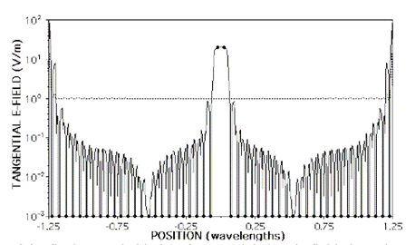
The magnitude of the finely sampled induced tangential electric field along the axis (the current is on the surface) of a 2.5-wavelength, 50-segment wire 10-3 wavelengths in radius modeled using NEC. For the antenna case (the solid line) the two 20-V/m source segments are obvious as are the other 48 match points (the solid circles) whose values are generally on the order of 10-13 or less. For the scattering problem, the scattered E-field (the dashed line) is graphically indistinguishable from the incident 1 V/m excitation except near the wire ends. The IEMF and far-field powers for the antenna are 1.257x10⁻² w and 1.2547x10⁻² w, respectively. For the scattering problem, the corresponding powers are 5.35x10⁻⁴ and 5.31x10⁻⁴ watts.
Two Novel Approaches to Antenna-Pattern Synthesis
Abstract
The design of linear arrays that produce a desired radiation pattern, i.e. the pattern-synthesis problem, continues to be of interest as demonstrated by the number of articles that continue to be published on this topic. A wide variety of approaches have been developed to deal with this problem of which two are examined here. One of them, a matrix-based method, begins with a specified set of element currents for a chosen array geometry. A convenient choice, for example, is for all of the current elements to be of unit amplitude. Given its geometry and currents, an initial radiation pattern for the array can be computed. A matrix is constructed whose individual coefficients are comprised of the contribution each element current makes to the various lobe maxima of this initial radiation pattern. Upon forming the product of the inverse of this matrix with a vector whose entries are the desired amplitudes of each maxima in the radiation pattern to be synthesized, a second set of element currents is obtained. The lobe maxima of the pattern that this second set of element currents generates usually change somewhat in angle relative to those of the initial pattern while their amplitudes will also not match those specified. The process is repeated as an iterative sequence of element-current and pattern computations. When the locations of the lobe maxima no longer change in angle and their maxima converge to the values specified the synthesis is complete. Results from this approach are demonstrated for several patterns an example of which follows below.

The pattern of a 15-element array synthesized to have a pattern increasing monotonically in 5 dB steps from left to right.
The second approach is based on a pole-residue model for an array whose element locations (the poles) and currents (the residues) are developed from samples of the specified pattern. One way of solving for the poles and residues is provided by Prony’s Method, and another is the Matrix-Pencil procedure. However found, the spacing between the array elements derived using such tools can in general be non-uniform, a potential advantage in reducing the problem of grating lobes. There are three parameters that need to be chosen for the pattern sampling: 1) the number of poles in the initial array model, for each of which two pattern samples are required; 2) the spacing of the pattern samples themselves, being required to be in equal steps of ![]() , with
, with ![]() the observation angle from the array axis; and 3) the total pattern window that is sampled. The pattern rank is an important parameter as it establishes the minimum number of elements that are needed for the array, and can be determined from the singular-value spectrum of the matrix developed from the pattern samples. The pole-residue approach is summarized and various examples its use are also demonstrated.
the observation angle from the array axis; and 3) the total pattern window that is sampled. The pattern rank is an important parameter as it establishes the minimum number of elements that are needed for the array, and can be determined from the singular-value spectrum of the matrix developed from the pattern samples. The pole-residue approach is summarized and various examples its use are also demonstrated.
Some Computational “Tricks of the Trade”
Abstract
Numerical computations have become ubiquitous in today’s world of science and engineering, not least of which is the area of what has come to be called computational electromagnetics. Students entering the electromagnetics discipline are expected to have developed a working acquaintance with a variety of numerical methods and models at least by the time they reach graduate studies, if not earlier in their undergraduate education. Most will have obtained some experience with the broader issues involved in numerically solving differential and integral equations. However, there are a variety of specialized numerical procedures that contribute to the implementation and use of numerical models that are less well known, and which form the basis for this lecture. Among such procedures are:
1) Acceleration techniques (e.g., Shank’s method, Richardson extrapolation, Kummer’s method) that enable estimating an answer for an infinite series or integral using many fewer terms;
2) Adaptive techniques such as one based on Romberg quadrature that permit more efficient numerical evaluation of integrals;
3) Model-based techniques that can reduce the number of samples needed to estimate a transfer function or radiation pattern.
4) “Backward” recursion that develop classical functions from noise together with an auxiliary condition.
5) Ramanujan’s modular-function formula for Pi whose accuracy increases quartically with each increase in the computation order.
This lecture will survey some of these procedures from the perspective of their applicability to computational electromagnetics. A specific example of an acceleration technique is the Leibniz series for pi, which provides N-digit accuracy after summing approximately 10N terms. Shank’s method, on the other hand provides N-digit accuracy after N terms of the Leibniz series as shown in the triangle array below.
4.000000000
2.666666666 3.166666666
3.466666666 3.133333333 3.142105263
2.895238095 3.145238095 3.141450216 3.141599357
3.339682539 3.139682539 3.141643324 3.141590860 3.141592714
2.976046176 3.142712843 3.141571290 3.141593231 3.141592637 3.141592654
3.283738484 3.140881349 3.141602742 3.141592438 3.141592659
3.017071817 3.142071817 3.141587321 3.141592743
3.252365935 3.141254824 3.141595655
3.041839619 3.141839619
3.232315809
A Personal Retrospective on 50 Years of Involvement in Computational Electromagnetics
Abstract
This presentation briefly reviews some selected aspects of the evolution and application of the digital computer to electromagnetic modeling and simulation from a personal perspective. First considered are some of the major historical developments in computers and computation, and projections for future progress. Described next are some of the author’s personal experiences in computer modeling and electromagnetics resulting from his research activities in industry, government laboratories and academia dating from introduction of the IBM 7094. Some aspects of the impact that computer modeling has had more generally on the discipline of computational electromagnetics (CEM) is then summarized. Issues of potential interest not only to CEM but also to scientific computing in general are then briefly considered. These include: 1) verification and validation of modeling codes and their outputs; 2) the importance of statistics and visualization as computer models become larger and more complex; and 3) some issues related to first-principles or micro-modeling and reduced-order or macro-modeling of physical observables and their connection with signal processing. Various illustrative examples are shown to demonstrate some of these issues with the talk concluding with a few personal remarks.

The growth of computer speed in FLOPs/sec since 1953. The cross marks the time of the author’s first involvement in computational electromagnetics.
Evolution of the Digital Computer and Computational Electromagnetics
Abstract
The development and evolution of the digital computer is a fascinating and still-unfolding story. This presentation briefly surveys this fascinating topic beginning with the origin of numbers and mathematics and concluding with present and anticipated future capabilities of computers in terms of their impact on computational electromagnetics (CEM). Numerous intellectual and technological breakthroughs over millennia have contributed to the current state-of-art. The development of arithmetic and computing might be said to begin with an ability to count. The first “recorded” number that has been found, a slash mark on the fibula of a baboon and apparently signifying the number 1 is about 20,000 years old. Counting and numbers eventually followed some 15,000 years later due to the Babylonians who invented the abacus as the first calculating tool at about the same time that the Egyptians introduced the first known symbols for numbers using a base-10 system. The number zero appeared about 500 CE in India with fractions and negative numbers coming a little later as did the Arabic number system, also credited to India.
It was about a thousand years later that the appearance of the first computational device beyond the abacus occurred, the “Pascaline” invented by Pascal for addition and subtraction in 1642. Leibniz added the capability for multiplication and division in 1671 with the “Leibniz wheel” which is still used in electromechanical calculators. Related computational developments include the invention by de Vaucanson of the punched wooden card for controlling a special loom that was later perfected by Jacquard. Babbage proposed his “difference” engine for calculating tables in 1822, followed in 1833 by his “analytical” engine, the first programmable computer. Punched cards were first used in a numerical setting by Hollerith for the 1890 US census with his company becoming part of IBM in 1911. The light bulb and the “Edison effect” began the electronics revolution with Fleming’s and De Forest’s work leading to the first triode in 1906.
The computer revolution began in earnest in the 1930s with a series of electromechanical computers due to Vennevar Bush at MIT, Konrad Zuse in Germany, and Howard Aiken with the IBM Mark 1. The latter was used during World War II for computing artillery-firing tables. The first all electric computer was built at Iowa State College by Atanasoff and Berry in 1939 and the first all electronic computer, Colossus, was developed in 1943-1944 in Britain for code breaking on a project headed by Alan Turing. A series of “AC” or “automatic computers” followed, such as ENIAC, EDSAC, ILLIAC I, ORDVAC, EDVAC and UNIVAC. The first transistor-based system, the IBM 7090, was introduced in 1959 with the IBM 7094 using ferrite-core memory following a few years later.
The onset of CEM can probably be said to date to the 1940’s using electromechanical calculators. These were still being used as late as 1960 at the Radiation Laboratory at the University of Michigan for computing tables of special functions and related quantities. The IBM 704 and 7094 soon took over this role that the author exploited in developing a computational thesis from 1963 to 1965. A special issue of the IEEE Proceedings in 1965 highlighted EM computations with the moment method popularized by the Harrington book in 1968. What were once considered “big” problems in the 1960’s using an integral-equation model having 200 or so unknowns have expanded to millions of unknowns now, even on personal computers, with an expanding set of tools and models. The growth rate in performance from the UNIVAC until now has been one of unparalleled progress, by a factor of 10 every 5 years. If this were to continue until 2053, computing speed will have grown to ~1023 FLOPS! ensuring a commensurate impact on CEM.


From the abacus to the IBM 7094 and beyond.
Biography
Since earning his PhD in Electrical Engineering at the University of Michigan, E. K. Miller has held a variety of government, academic and industrial positions. These include 15 years at Lawrence Livermore National Laboratory where he spent 7 years as a Division Leader, and 4+ years at Los Alamos National Laboratory from which he retired as a Group Leader in 1993. His academic experience includes holding a position as Regents-Distinguished Professor at Kansas University and as Stocker Visiting Professor at Ohio University. Dr. Miller wrote the column “PCs for AP and Other EM Reflections” for the AP-S Magazine from 1984 to 2000. He received (with others) a Certificate of Achievement from the IEEE Electromagnetic Compatibility Society for Contributions to Development of NEC (Numerical Electromagnetics Code) and was a recipient (with others) in 1989 of the best paper award given by the Education Society for “Computer Movies for Education.”
He served as Editor or Associate Editor of IEEE Potentials Magazine from 1985 to 2005 for which he wrote a regular column “On the Job,” and in connection with which he was a member of the IEEE Technical Activities Advisory Committee of the Education Activities Board and a member of the IEEE Student Activities Committee. He was a member of the 1992 Technical Program Committee (TPC) for the MTT Symposium in Albuquerque, NM, and Guest Editor of the Special Symposium Issue of the IEEE MTT Society Transactions for that meeting. In 1994 he served as a Guest Associate Editor of the Optical Society of America Journal special issue “On 3 Dimensional Electromagnetic Scattering.” He was involved in the beginning of the IEEE Magazine "Computing in Science and Engineering" (originally called Computational Science and Engineering) for which he has served as Area Editor or Editor-at-Large. Dr. Miller has lectured at numerous short courses in various venues, such as Applied Computational Electromagnetics Society (ACES), AP-S, MTT-S and local IEEE chapter/section meetings, and at NATO Lecture Series and Advanced Study Institutes.
Dr. Miller edited the book "Time-Domain Measurements in Electromagnetics", Van Nostrand Reinhold, New York, NY, 1986 and was co-editor of the IEEE Press book Computational Electromagnetics: Frequency-Domain Moment Methods, 1991. He was organizer and first President of the Applied Computational Electromagnetics Society (ACES) for which he also served two terms on the Board of Directors. He served a term as Chairman of Commission A of US URSI and is or has been a member of Commissions B, C, and F, has been on the TPC for the URSI Electromagnetic Theory Symposia in 1992 and 2001, and was elected as a member of the US delegation to several URSI General Assemblies. He is a Life Fellow of IEEE from which he received the IEEE Third Millennium Medal in 2000 and is a Fellow of ACES. His research interests include scientific visualization, model-based parameter estimation, the physics of electromagnetic radiation, validation of computational software, and numerical modeling about which he has published more than 150 articles and book chapters. He is listed in Who's Who in the West, Who's Who in Technology, American Men and Women of Science and Who's Who in America.